Block-Subunit Diffusion Priors for
High-Dimensional Tabular Data Generation
Learn global dependence in a compact space of block subunits,
then decode high-dimensional synthetic samples with realistic
marginals, dependencies, and optional missingness.
Al Zadid Sultan Bin Habib · Md Younus Ahamed ·
Prashnna Kumar Gyawali · Gianfranco Doretto ·
Donald A. Adjeroh
10Distinct generator baselines across the evaluation
89.21%Extended nine-dataset mean TSTR AUC, no-permutation variant
Browse page sections
Paper Abstract
Abstract
High-Dimensional Low-Sample Size (HDLSS) tabular domains
(e.g., omics) are characterized by \(n \ll m\), where
\(n\) = number of samples, and \(m\) = number of features.
Such domains often exhibit strong local correlation groups,
sparse cross-group dependencies, heavy-tailed non-Gaussian
marginals, heteroscedastic noise, and structured missingness,
making direct density learning in \(\mathbb{R}^m\)
ill-conditioned since \(n \ll m\).
We propose BSTabDiff, a block-subunit
generative framework that partitions the \(m\) observed
features into \(M\) latent blocks (\(M \ll m\)) and
generates each block via a shared low-dimensional subunit
variable, concentrating global dependence learning in the
compact block-latent space \(\mathbb{R}^M\) while decoding
to the full feature space with copula-driven dependence,
flexible per-feature marginals, and explicit missingness
mechanisms. BSTabDiff can induce a data-driven feature
ordering and block construction before latent partitioning,
allowing the model to better align with local dependency
structure when such organization is beneficial. BSTabDiff
supports modern deep priors on block latents, including
diffusion and normalizing flows, enabling stable synthesis
and controllable benchmark generation in the HDLSS regime.
Empirically, BSTabDiff produces more realistic and more
stable high-dimensional synthetic data when compared with
unstructured tabular generators on HDLSS data.
Motivation and Contributions
Why Block-Subunit Generation?
Conventional tabular generators often model relationships
over all features at once. When there are only dozens
or hundreds of samples but thousands of columns,
learning dense dependence becomes ill-conditioned.
BSTabDiff identifies groups of related features and
learns how those groups interact through shared factors.
\[
X \in \mathbb{R}^{m},
\quad
h=(h_1,\ldots,h_M)\in\mathbb{R}^{M},
\quad M\ll m,\quad n\ll m
\]
Full-dimensional observations, compact block-latent dependence.
Block-subunit model
Each related feature group shares one latent variable.
Deep latent prior
Diffusion or normalizing flows model cross-block dependencies.
Structured decoding
Copula variables, marginal transforms, and missingness.
Feature ordering
GO-BS estimates column order and contiguous block boundaries.
HDLSS-oriented analysis
Block factorization, identifiability, and sample efficiency.
Sustainable learning
Utility, fidelity, compute, energy, and carbon evaluation.
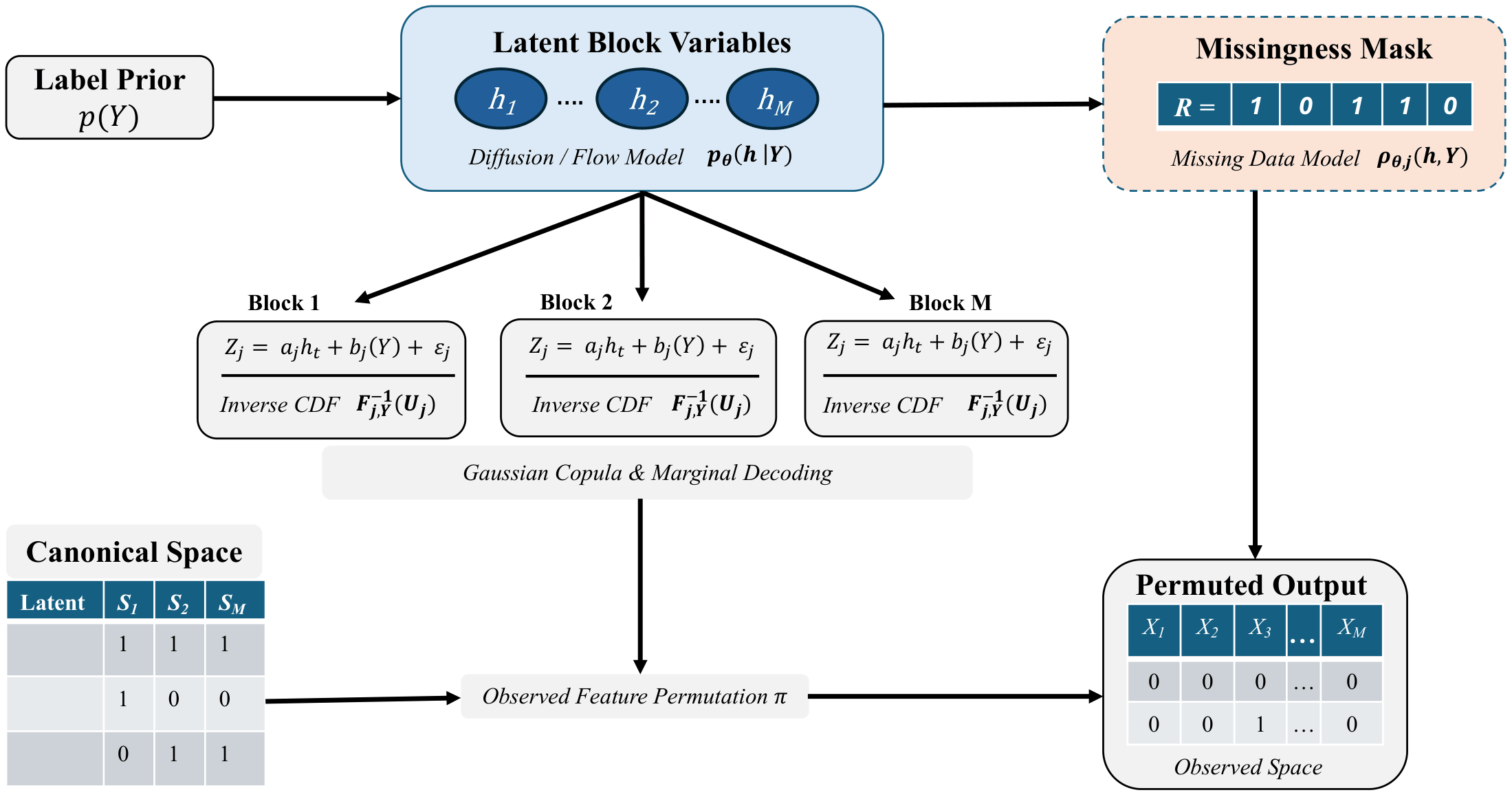
Architecture
End-to-End Generative Pipeline
BSTabDiff separates block-level dependence learning
from full-dimensional feature emission. The architecture
integrates optional class conditioning, diffusion/flow
priors, missingness, inverse marginal decoding, and
observed-feature permutation.
Optional class prior
Draw a label \(Y \sim p(Y)\), or fix a class
for conditional generation.
Sample compact block latents
Draw \(h \sim p_\theta(h\mid Y)\) from a
diffusion or flow prior.
Generate observation mask
Construct \(\widetilde R \in \{0,1\}^{m}\) from a
feature-specific missingness process.
Decode each feature
Use block-conditioned Gaussian copula variables
and learned inverse marginal CDFs.
Restore feature order
Return generated features to their observed
indexing when ordering has been applied.
Core Methodology
Explore the Mathematical Formulation
Select a stage to explore BSTabDiff's six-part
generative formulation. The equations describe
the methodology, while the interactive diagrams
provide conceptual illustrations rather than
outputs from a trained model.
Step 1 of 6
Latent Block Partition
Let canonical feature indices be divided into
M disjoint blocks. Features in the same block
share the latent subunit hₜ.
Instead of learning dependencies directly
across all m features, BSTabDiff learns
global dependence among M block latents.
Conceptual block illustration
A toy example with 12 features.
Adjust M to change the partition.
Mathematical notation is rendered using MathJax.
The interactive illustrations demonstrate the
methodology conceptually.
Structure-Aware Learning
Graph-guided Ordering with Block Segmentation
GO-BS constructs a weighted
feature-affinity graph and searches for a feature
permutation and contiguous block boundaries
that keep strongly dependent features together.
Within-block affinity is rewarded, cross-block affinity
is penalized, and the block size regularizer
\(\Omega(b)\) controls the resulting partition structure.
Interactive Feature Ordering Explorer
Eight toy features form two planted correlation groups
(blue and peach).
Select any two feature chips to swap their positions.
Reordering updates the affinity matrix display and
recalculates the within-block, cross-block, and
objective scores.
Feature Order & Affinity Matrix
Darker squares mean higher affinity \(W_{ij}\).
Blue dividers mark block boundaries.
Diagonal cells are omitted.
Live Objective Breakdown
Within-block affinity ↑—
Cross-block affinity ↓—
Boundary regularizer (toy Ω)—
Number of boundaries—
Illustrative objective J (lower is better)
—
Important:
This is an educational example, not the trained
GO-BS optimizer. Its boundary surrogate is
\(\Omega_{\mathrm{toy}}(b)=M-1\);
it does not claim that the paper uses this
particular regularizer. Affinities and group
memberships are illustrative.
Counts each unordered pair of features once
when they fall in different blocks.
Here, \(B_t(\pi,b)\) denotes the t-th contiguous
feature block, \(W_{ij}\) is the affinity between
features i and j, and \(\lambda\) and \(\gamma\)
control the cross-block and boundary terms.
The objective corresponds to Eq. 10 of the
NeurIPS 2026 paper.
GO-BS
Sample-clustered graph ordering for coherent
feature block construction.
GO-BS-FC
Feature-clustered variant offering improved
compute–structure trade-offs in extreme dimensions.
Feature ordering can be optional. Where local feature
structure is weak, ordering may add computation
without improving utility. On the Cell Cycle
dataset (42,728 features),
GO-BS-FC achieved the strongest
TSTR performance among the evaluated variants.
Theory and Interpretation
Why BSTabDiff Helps in HDLSS
BSTabDiff leverages compact block-latent representations
and shared within-block structure to improve modeling
in High-Dimensional, Low-Sample Size (HDLSS) settings.
The theoretical analysis studies block identifiability
and the benefits of signal aggregation under specific
assumptions.
1. Compact Latent Modeling
Instead of learning global dependencies directly
across all \(m\) observed features, BSTabDiff
concentrates dependence learning in
\(M\) block latents, where \(M \ll m\).
100×
Fewer global dependence coordinates
in the block-latent representation
Original feature space10,000
Block-latent space100
\[
X\in\mathbb{R}^{m},
\qquad
h\in\mathbb{R}^{M},
\quad M\ll m
\]
The ratio \(m/M\) represents the reduction
in dependence-space dimensionality.
It is not a guaranteed reduction in
runtime, memory use, or parameter count.
2. Signal Aggregation
When features within a block share a class-dependent
mean shift and have independent Gaussian noise,
averaging them reduces conditional variance
and improves signal-to-noise ratio.
Illustrative assumptions:
\(\mu_1-\mu_0=1\) and \(\sigma=2\).
Simplified mean-shift Gaussian example
corresponding to Lemma 3.5.
Increasing \(s\) improves SNR linearly
under the stated assumptions;
correlated noise or heterogeneous
feature signals can change this behavior.
Theoretical interpretation.
The paper investigates identifiability of
block structure up to block-label permutations
under distinct block-dependence assumptions.
The GO-BS optimization objective is NP-hard,
motivating approximate solvers.
These results and sample-efficiency
interpretations are conditional on their
stated assumptions rather than universal
guarantees.
Experimental Evaluation
TSTR vs TRTR · 18 Datasets
TSTR = Train on Synthetic, Test on Real;
TRTR = Train on Real, Test on Real.
Bars show the highest reported mean BSTabDiff TSTR
for each dataset alongside the real data reference.
Use the controls to switch between
Accuracy and ROC-AUC.
Evaluation Metric
Primary HDLSS · Accuracy
BSTabDiff TSTR
Real TRTR
0255075100%
Figure: BSTabDiff synthetic data utility compared
with training on real data. Each bar uses a fixed
0–100% scale. Variant labels identify the selected
configuration. Accuracy and AUC are shown separately.
Dataset Dimensions
n = samples; m = features.
Dataset
n
m
Sources: BSTabDiff (NeurIPS 2026), Tables 2 and 4,
and Appendix Tables A8.1, A18.1, and A23.3.
Results show dataset-level means; standard
deviations are provided in the paper.
CIFAR-10 uses ResNet-50 image embeddings;
Springleaf uses the processed subset.
The best variant may differ across datasets.
Compute and Sustainability
Efficiency and Responsible Interpretation
Compact prior
Learn cross-block dependence in \(M\)
latent variables, not all \(m\) features.
Fast HDLSS synthesis
Reported no-permutation runs typically
finish in under 10 seconds on Vulcan (NVIDIA RTX A6000) hardware.
Energy-carbon analysis
The evaluation measures utility, energy,
CO₂e, memory, and computational cost.
Emission fitting scales with observed
sample-feature entries, while the main
diffusion dependence-learning cost depends
on the smaller latent dimension \(M\).
GO-BS preprocessing may add significant
computation in extreme feature spaces.
BSTabDiff is designed primarily for HDLSS data.
Synthetic data should complement, rather
than replace, real data validation and
expert review. Fidelity and downstream
utility remain dataset dependent, and
the method does not imply formal
differential privacy.
Open-Source Implementation
Installation and Reproducibility
BSTabDiff is available on PyPI and can be installed
directly using pip. Source code, notebooks, smoke tests,
and experimental instructions are available in the
GitHub repository.
BSTabDiff was previously presented at the
ICLR 2026 DeLTa Workshop
and subsequently accepted as a
NeurIPS 2026 main conference poster.
Please cite the NeurIPS version for the
main conference publication.
This work was supported in part by
the US National Science Foundation (NSF)
under Awards
1920920,
2125872,
2223793,
and
2318708.
NeurIPS 2026 Review Process
We sincerely thank the anonymous NeurIPS 2026
reviewers for their valuable feedback and
constructive suggestions. We are especially
grateful to the anonymous Area Chair for their
thoughtful insights and guidance, which
significantly contributed to strengthening
this work.
If you use BSTabDiff or its published results,
please cite our NeurIPS 2026 paper.
@inproceedings{habib2026bstabdiff,
  title     = {BSTabDiff: Block-Subunit Diffusion Priors for High-Dimensional Tabular Data Generation},
  author    = {Habib, Al Zadid Sultan Bin and Ahamed, Md Younus and Gyawali, Prashnna Kumar and Doretto, Gianfranco and Adjeroh, Donald A.},
  booktitle = {Advances in Neural Information Processing Systems (NeurIPS)},
  year      = {2026}
}